You have a pump curve in front of you — or a supplier has just sent you one — and you need to confirm whether the pump will do what your system needs. Or your pump has been underperforming and you want to understand where on the curve it is actually running. Either way, this guide gives you the practical ability to read, interpret, and use pump performance curves to make real engineering decisions.
Pump curves are not complicated once you understand what each line is telling you. A pump curve is the manufacturer’s promise of what the pump will do — how much head it will produce at each flow rate, at what efficiency, consuming how much power, and requiring how much suction pressure. Reading it correctly is the difference between selecting a pump that runs near its Best Efficiency Point for 15 years, and selecting one that operates off-curve, cavitates, and destroys itself in 18 months.
This guide covers every line on a standard pump performance curve, how to construct a system curve, how to find the true operating point, and how VFDs and multi-pump arrangements change the picture — with two worked examples drawn from Australian industrial applications.
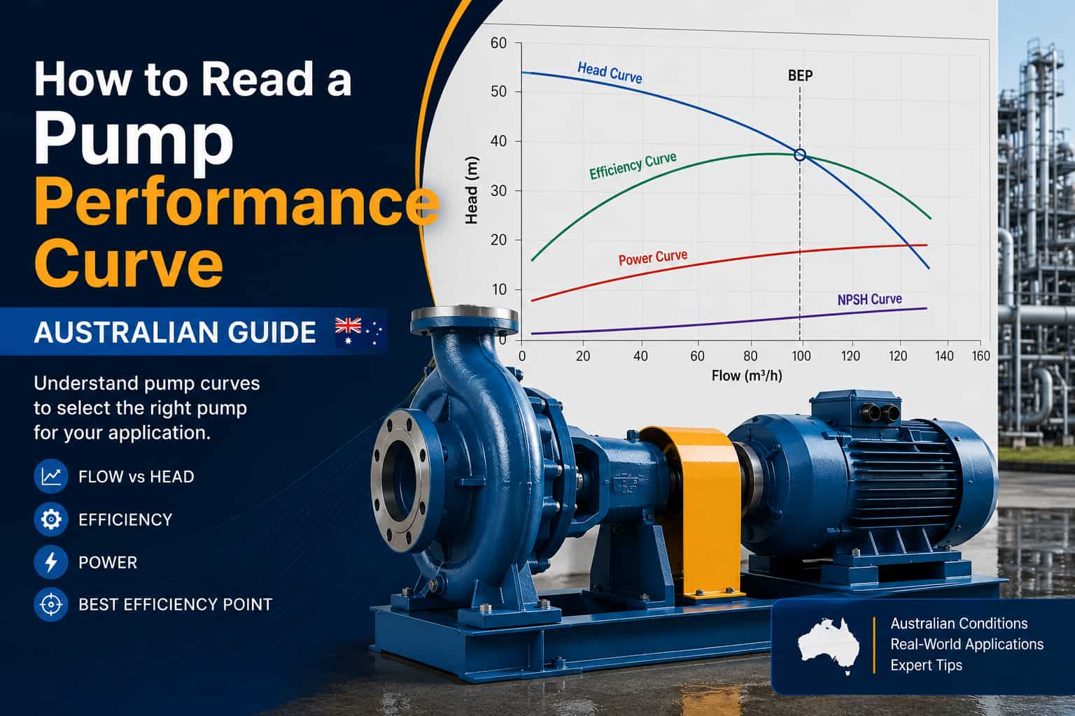
A pump performance curve is a graphical representation, published by the pump manufacturer, of how a specific pump behaves across a range of flow rates at a fixed speed and impeller diameter. A standard curve sheet combines four curves plotted against flow rate on the horizontal axis: the H-Q curve (head vs flow); the efficiency curve (η %); the power curve (kW); and the NPSHr curve (minimum suction head required). The pump curve is the primary tool for every pump selection, performance check, and troubleshooting decision.
1. Anatomy of a Pump Performance Curve — All Four Lines Explained
A standard pump datasheet contains four separate curves, all plotted against the same horizontal axis — flow rate (Q, in L/s or m³/hr). Each curve answers a different engineering question. Here is what each one tells you.
(Head vs Flow)
The main curve — shows how much total dynamic head (metres) the pump produces at each flow rate (L/s or m³/hr). Head decreases as flow increases. This is the pump’s fundamental performance signature. Plotted on the primary Y-axis (left).
(η vs Flow)
Shows the pump’s hydraulic efficiency (%) at each flow rate. Starts low at zero flow, rises to a peak (the BEP), then falls at high flow. The peak of this curve is the most important single point on the chart. Plotted on the secondary Y-axis (right) or on the same axis as head.
(kW vs Flow)
Shows the shaft power (kW or BHP) consumed by the pump at each flow rate. Typically rises with flow rate. Use this curve to confirm the selected motor is not undersized at any operating point — particularly at maximum expected flow (run-out). Motor kW must exceed the peak power curve value with at least 10% margin.
(m vs Flow)
Shows the minimum suction head (metres) the pump requires to prevent cavitation at each flow rate. NPSHr rises as flow increases. Always check NPSHr against your system’s available NPSHa — particularly at maximum expected flow, not just design flow. Your system must always deliver NPSHa ≥ 1.1 × NPSHr.
All pump performance curves are generated by the manufacturer using clean water at approximately 20°C at sea level on a test rig, at the exact impeller diameter specified. Real-world performance deviates when: the fluid is more viscous than water (reduces head, flow, and efficiency — requires viscosity correction); the fluid is less dense (reduces head in pressure terms but not in metres); the pump is installed at elevation (reduces atmospheric pressure, reducing NPSHa); or the impeller has been trimmed or has worn. Always apply corrections for your actual fluid and conditions — do not use water-test curves without adjustment for viscous or dense fluids.
2. The H-Q Curve in Depth — Reading the Pump’s Head-Flow Relationship
The H-Q curve (also called the head-flow curve or performance curve) is the primary line on the chart. It defines the pump’s behaviour: as flow increases, head decreases. This inverse relationship is fundamental to centrifugal pump operation — a centrifugal pump is a head-producing device, and the head it can produce depends entirely on how much fluid is flowing through it.
Three Critical Points on the H-Q Curve
| Point | Location on curve | What it means | Risk if operated here |
|---|---|---|---|
| Shut-off head | Far left — zero flow, maximum head. Discharge valve closed | Maximum head the pump can produce. All input energy converts to heat in the fluid | High — overheating of pump casing and fluid. Acceptable for brief start-up only; not for continuous operation |
| BEP | Middle of curve — at the peak of the efficiency curve | The design point — maximum efficiency, minimum internal turbulence and mechanical stress | Low — this is where the pump is designed to run. Target the system curve to intersect here |
| Run-out (end of curve) | Far right — maximum flow, minimum head. Fully open discharge with low system resistance | The pump is producing maximum flow — motor is at or above rated power, NPSHr is at its highest | High — motor overload risk, cavitation from high NPSHr, mechanical stresses from off-BEP turbulence |
Steep vs Flat H-Q Curves — Which Suits Your Application?
Head drops sharply as flow increases. Preferred for systems with variable resistance — mine dewatering sumps with varying water level, water supply networks with variable demand. A steep curve means the operating point moves significantly in flow when system resistance changes, which helps the pump self-regulate. Also preferred for parallel pump installations to prevent flow imbalance between pumps.
Head remains relatively constant across a wide flow range. Preferred for systems with stable resistance and precise flow control requirements — food and beverage process lines, chemical dosing circuits, boiler feed systems. A flat curve delivers nearly constant pressure across a wide flow range. Also suits systems where pump head must match a fixed downstream pressure setpoint.
3. The BEP — The Most Important Single Point on the Entire Curve
The Best Efficiency Point (BEP) is the flow rate at which the pump runs most efficiently with the least internal turbulence and vibration. It is the peak of the efficiency curve — the point at which the pump converts the maximum proportion of motor input power into useful hydraulic energy. Selecting a pump that operates at or near BEP is not just an efficiency decision — it is a reliability and service life decision.
When a centrifugal pump operates significantly away from BEP, internal flow patterns deviate from the impeller’s design geometry. Fluid approaches the impeller vanes at the wrong angle, generating turbulence, separation, and recirculation zones within the pump. This internal turbulence causes:
Recirculation cavitation pits impeller vane surfaces
Elevated radial thrust at low and high flow extremes
Shaft vibration from off-BEP hydraulics damages seal faces
Hydraulic turbulence generates audible noise and structural vibration
Lower efficiency = more kW consumed for the same output
Operating Regions — HI Standard
| Region | Flow range (% of BEP) | Status | Notes |
|---|---|---|---|
| Preferred Operating Region (POR) | 80–110% of BEP flow | ✓ Target this | Maximum efficiency, minimum mechanical stress, longest service life. Select pump so that expected operating point falls within this range |
| Allowable Operating Region (AOR) | 70–120% of BEP flow | ⚠ Acceptable short-term | Acceptable for continuous operation but with some efficiency and life penalty. Average operating point should be within POR |
| Outside AOR — low flow | <70% of BEP flow | ✗ Avoid continuous | Internal recirculation at impeller eye — pitting, vibration, bearing and seal damage. Install minimum flow bypass or VFD |
| Outside AOR — high flow | >120% of BEP flow | ✗ Avoid continuous | Motor overload risk, high NPSHr may exceed NPSHa causing cavitation, discharge recirculation, high radial thrust |
4. The System Curve — Finding the True Operating Point
The pump curve alone cannot tell you where a pump will actually operate. You need the system curve — a plot of the total head required by your piping system at each flow rate. The true operating point is where the pump curve and the system curve cross.
The pump will operate at the intersection of the pump curve and system curve. A constant speed pump only has this head curve available and will track up and down it as the system curve changes.
How to Draw a System Curve
What Changes the System Curve — and How It Moves the Operating Point
| System change | Effect on system curve | Effect on operating point |
|---|---|---|
| Throttle discharge valve | System curve steepens (more friction at each flow) | Operating point moves left — lower flow, higher head. Pump operates left of BEP. Energy wasted in valve |
| Open discharge valve / reduce friction (new pipe, larger pipe) | System curve flattens (less friction at each flow) | Operating point moves right — higher flow, lower head. Risk of operating beyond AOR right boundary |
| Pipe scale/corrosion (friction increases over time) | System curve gradually steepens over years of service | Operating point gradually moves left — flow slowly declines without any pump change. Very common cause of “pump performance declining” complaints |
| Raise discharge tank level / increase downstream pressure | Static head (Hstatic) increases — system curve shifts up uniformly | Operating point moves left — lower flow at same pump speed. Relevant for variable-level tanks and variable-pressure downstream systems |
5. The NPSHr Curve — Confirming Your System Won’t Cavitate
NPSHr is the minimum amount of pressure required on the suction side of the pump to avoid cavitation. It is a property of the pump — it rises as flow increases — and it must always be compared against the NPSHa of your system. If NPSHa falls below NPSHr at any expected operating flow, the pump will cavitate.
The critical mistake most engineers make when checking NPSH is checking it only at the design flow — not at the maximum expected flow. As flow increases toward run-out, NPSHr rises sharply on the pump curve. A pump with comfortable NPSH margin at design flow may have insufficient margin if system conditions allow flow to exceed the design point. Always verify NPSHr at the maximum possible operating flow, not just the design point.
Calculated from your installation. NPSHa = (Patm – Pvapour) ÷ (ρg) + Hs – hf. Depends on liquid level, suction pipe size, fluid temperature, and elevation. Always compare at worst-case conditions — minimum suction level, maximum fluid temperature, dirtiest strainer condition.
Read directly from the pump curve at the operating flow rate. The minimum inlet pressure (metres) the pump needs to avoid cavitation. Determined by impeller geometry — cannot be changed without changing the impeller or reducing pump speed.
If your system’s NPSHa is insufficient for the selected pump, the solutions are: choose a pump with lower NPSHr for the same duty (inducer pump, lower-speed design, double-suction impeller); increase NPSHa by raising the liquid level, lowering the pump, widening the suction pipe, or reducing fluid temperature; or reduce pump speed with a VFD (NPSHr decreases with speed). For complete guidance on cavitation diagnosis and NPSH calculation, see our pump cavitation guide.
6. Affinity Laws and VFD Speed Curves — How Speed Changes the Pump Curve
When a pump is fitted with a Variable Speed Drive (VSD/VFD), the operating speed changes — and the entire pump curve shifts according to the Affinity Laws. Understanding how the curve moves allows you to predict the pump’s performance at any speed and identify the new operating point without retesting the pump.
VFD Worked Calculation — Australian Mine Dewatering Pump
A mine dewatering centrifugal pump rated at 1,450 RPM produces 45 L/s at 65m head, consuming 45 kW. The Bowen Basin mine site wants to reduce dewatering rate in the dry season (low inflows) — how does the pump perform at 1,160 RPM (80% of rated speed)?
New head: H₂ = 65 × (0.80)² = 65 × 0.64 = 41.6 m
New power: P₂ = 45 × (0.80)³ = 45 × 0.512 = 23.0 kW
VFDs are not lossless — they introduce 2–3% efficiency losses at full speed and become less efficient as load drops. At very low speeds, actual pump efficiency can fall meaningfully below what the Affinity Laws predict. Industry practice limits VFD pump operation to a minimum of 30% of rated speed (some applications 50%) below which pump hydraulic efficiency collapses and minimum flow requirements for bearing cooling and seal lubrication may not be met. Always set a minimum speed setpoint on the VFD — do not allow the pump to run at arbitrarily low speeds without checking performance at that speed point.
7. Parallel and Series Pump Curves — Combined Performance
When two or more pumps are installed in the same system, their combined performance must be calculated from the individual curves — the combined curve is not the same as doubling a single pump’s output in all situations.
Pumps in Parallel
How to combine: At each head value on the curves, add the flow rates together. The combined parallel curve shows double the flow at each head (for two identical pumps).
Actual outcome: Assuming two identical pumps, flow rate doubles when used in parallel. However, the actual increase in flow is less than double — higher combined flow increases friction losses, the system curve curves upward, and the operating point shifts to a higher flow but lower head per pump on the individual pump curves.
Best for: High-flow, low-to-moderate static head systems — water supply networks, mine dewatering sump circuits with multiple pumps, large food processing CIP flow requirements.
⚠ With parallel pumps: verify that each individual pump, when the other trips, does not move past the AOR right boundary on the single-pump curve.
Pumps in Series
How to combine: At each flow rate value on the curves, add the head values together. The combined series curve shows double the head at each flow (for two identical pumps).
Actual outcome: Each pump adds its head contribution to the total. The actual flow is determined by where the combined series curve intersects the system curve — not simply double the head at the original flow.
Best for: High-head, moderate-flow systems — high-rise building water supply, multistage pipeline pumping, multistage centrifugal pump applications, reverse osmosis feed circuits.
⚠ With series pumps: if one pump trips, the remaining pump must have a bypass path to avoid dead-heading against the stopped pump’s check valve.
8. Impeller Trimming — Permanently Adjusting the Pump Curve
If a pump consistently operates to the right of its BEP — the operating point is at higher flow and lower head than the BEP — it may be oversized for the system. One permanent solution is impeller trimming: reducing the impeller outer diameter by machining, which shifts the pump curve down and to the left.
Impeller trimming is used when: the pump was oversized at specification (common when conservative safety margins were applied during system design); the system has changed since pump selection (reduced flow requirement, changed pipeline routing); or the pump was selected at a future expanded capacity and the current system does not need full flow.
Impeller Trim Calculation
Where D₁ = original impeller diameter, D₂ = trimmed diameter. The Affinity Laws for diameter changes are less accurate for large trims (>15% reduction) — always verify with the pump manufacturer before machining. Trimming is permanent — calculate carefully before cutting.
For systems with constant flow requirements: impeller trimming is the lower-cost permanent solution — one-time machining cost with no ongoing electrical losses. For systems with variable flow requirements: a VFD is better — it can adjust speed continuously to match demand and offers the energy savings of the Affinity Laws cube relationship. For systems that will be expanded in future: maintain the original impeller and use a VFD now — the full impeller can be used at higher speed when the system grows. Contact Pump Power Australia for a cost-benefit comparison for your specific system.
9. Two Worked Examples — Australian Industrial Applications
Example 1 — Selecting a Pump from a Curve: Brisbane Food Processing CIP Circuit
Step 1 — Locate design point on the curve:
Find 12 L/s on X-axis, 22m on Y-axis. Confirm this point sits on or below the pump’s H-Q curve. If the curve passes above this point — the pump produces more head than needed at 12 L/s, meaning the actual operating point (with system curve) will be at higher flow than 12 L/s.
Step 2 — Construct system curve:
Hstatic = 8m. k = 14 ÷ 12² = 0.0972. Calculate at several flows: Q=6: H = 8 + 0.0972×36 = 11.5m. Q=9: H = 8 + 0.0972×81 = 15.9m. Q=12: H = 22m. Q=15: H = 8 + 0.0972×225 = 29.9m. Plot these points — this is the system curve.
Step 3 — Find true operating point:
Identify where the system curve crosses the pump H-Q curve. If this occurs at 13.5 L/s and 23m — the pump is operating slightly right of the design point. Check efficiency at 13.5 L/s — if this is within the Preferred Operating Region (80–110% of BEP flow), the pump selection is acceptable.
Step 4 — Check NPSHr at 13.5 L/s:
Read NPSHr from the pump curve at 13.5 L/s — say 2.8m. Calculate NPSHa for the system at 45°C. Vapour pressure of water at 45°C = 9,593 Pa. NPSHa = (101,325 – 9,593) ÷ (990 × 9.81) + 1.0 – 0.8 = 9.46 + 0.2 = 9.66m. NPSHa/NPSHr = 9.66/2.8 = 3.45 — well above 1.1 minimum. NPSH is comfortable for this food plant application.
Step 5 — Confirm motor power:
Read power curve at 13.5 L/s — say 4.8 kW. Motor selection should be at least 5.3 kW (10% margin). Standard selection: 5.5 kW motor. For a food and beverage CIP circuit, confirm the pump uses stainless steel and food-grade seal materials — this is a centrifugal pump application suitable for a hygienic centrifugal design.
Example 2 — Troubleshooting a Declining Performance Pump: Perth Water Treatment Plant
A water treatment plant centrifugal pump at a Perth facility has shown gradually declining flow over 3 years — originally delivering 28 L/s, now only achieving 21 L/s despite no change to pump speed or system. The pump curve shows design BEP at 28 L/s, 35m. What has happened?
Diagnosis Step 1 — Has the system curve changed?
Measure suction and discharge pressure at the pump during operation. Calculate current friction losses (differential pressure minus static head). Compare to original commissioning data. If friction losses are significantly higher than 3 years ago — the system curve has risen due to pipe scaling, partial valve closure, or blocked strainer. The operating point has moved left on the same pump curve, reducing flow.
Diagnosis Step 2 — Has the pump curve degraded?
If system friction losses are unchanged but flow has still declined — the pump curve itself has dropped. Impeller wear, increased wear ring clearance, or internal corrosion all reduce the head produced at each flow rate. Measure differential pressure across the pump at a known flow — compare to the original pump curve. If the pump now produces less head at the same flow than its published curve, the impeller or wear rings need inspection.
Resolution:
In this Perth water treatment case — cleaning the pipe scale on the suction line and replacing a partially blocked strainer (confirmed by elevated strainer ΔP) reduced system friction losses back to near-original, restoring flow to 26 L/s. Remaining shortfall of 2 L/s traced to increased wear ring clearance from 3 years of operation — wear rings replaced at next scheduled shutdown, restoring full 28 L/s delivery. See our pump maintenance checklist for wear ring clearance measurement guidance.
10. Common Pump Curve Reading Mistakes — and How to Avoid Them
If your design point (Q=12 L/s, H=22m) sits on the pump curve but the system curve intersects the pump curve at Q=15 L/s — the pump will actually deliver 15 L/s, not 12 L/s. This can overload the motor, move the operating point outside the AOR, and cause cavitation if NPSHr at 15 L/s exceeds NPSHa. Always draw the system curve.
NPSHr rises steeply at high flow. A pump with adequate NPSH margin at 12 L/s design flow may cavitate badly if the system allows the operating point to move to 16 L/s on a low-resistance day. Check NPSHr at maximum possible flow — the far right of your expected operating range.
All pump curves are generated with water. For fluids more viscous than water — oils, syrups, slurries, concentrated chemicals — head, flow, and efficiency are all reduced compared to the water curve. The HI viscosity correction method (or Hydraulic Institute charts) must be applied before using the curve for selection. For gear pump and PC pump applications with viscous fluids, the curve corrections are particularly important.
A trimmed impeller or worn impeller no longer matches the published curve. If the curve on the datasheet is for 250mm diameter and the impeller has been trimmed to 235mm or has worn to an effective smaller diameter, the pump performance is lower than the curve shows. Always record the actual installed impeller diameter and recalculate expected performance using the Affinity Laws diameter relationship.
Engineers sometimes specify 15–20% head margin “for safety” — but this shifts the operating point left of BEP, into the region where recirculation and cavitation occur. A pump selected with the design operating point at 80% of BEP flow (to allow margin) may actually damage itself in normal operation. The correct approach is to calculate realistic system head at design flow and select a pump whose BEP falls at that duty — then verify the AOR covers any system variation, not select a pump that runs left of BEP by design.
11. Reddit and Quora Pump Curve Questions — Answered
These are the most frequently asked pump curve questions across Reddit r/ChemicalEngineering, r/mechanical_engineering, and Quora engineering communities — with direct answers.
The most common causes: (1) Actual system friction losses are higher than you calculated — check for partially closed valves, blocked strainer, scaled pipes. The system curve is steeper than designed, moving the operating point left. (2) The impeller has worn — measure differential pressure across the pump at a known flow and compare to the published curve. If the pump produces less head than the curve shows at that flow, the impeller has degraded. (3) The pump is running at lower than rated speed — confirm motor RPM or VFD frequency setting. (4) The fluid density or viscosity has changed from what the curve assumes — recalculate for actual fluid properties.
Yes — opening the discharge valve reduces system resistance, the system curve flattens, and the operating point moves right (higher flow, lower head) on the pump H-Q curve. But check two things before doing this: (1) The new operating point must stay within the pump’s Allowable Operating Region (maximum ~120% of BEP flow). Beyond this, motor overload and cavitation risk increase significantly. (2) NPSHr at the higher flow must remain below NPSHa. If the pump is already at the right edge of its curve, opening the valve further may cause damage rather than more useful flow. If flow is genuinely insufficient, consider parallel pump operation or a larger pump — not running an existing pump past its AOR.
Several possibilities even when the operating point appears correct on the curve: (1) The published curve is for the original impeller diameter — if the impeller has been trimmed or worn, the actual BEP may have shifted. (2) The flow reading is inaccurate — verify with a portable flow meter. (3) NPSHa is marginal — even when flow appears at BEP, if NPSHa is close to NPSHr, intermittent cavitation can cause noise and vibration. (4) Misalignment — shaft misalignment between pump and motor causes vibration at all operating points, not related to the curve. Check alignment. (5) Bearing failure — deteriorating bearings cause vibration regardless of operating point. Check bearing temperature and vibration levels. For detailed cavitation diagnosis, see our pump cavitation guide.
This is one of the most common conceptual confusions with centrifugal pumps. A centrifugal pump adds a fixed amount of energy (head) to the fluid — but how that energy is distributed between velocity and pressure depends on how much fluid is flowing. At zero flow (shut-off), all the energy appears as pressure (maximum head). As flow increases, more energy goes into accelerating the fluid through the pump and piping, and less is “left over” as pressure head at the outlet. The energy input from the motor is relatively constant, but friction losses within the pump itself increase with flow — so less net head is available at the discharge at higher flows. This is why centrifugal pump H-Q curves always slope downward from left to right.
This is normal and expected. The cubic relationship between power and speed means even modest speed reductions yield substantial energy savings. But the parallel pump benefit depends heavily on the system curve. In a high-friction, low-static-head system — where the system curve rises steeply — adding a parallel pump significantly increases friction losses at the higher combined flow, so the operating point on each individual pump shifts to lower head than the original single-pump operating point. The resulting flow increase may be only 20–40% above the single pump, not 100%. To maximise parallel pump flow gain: reduce system friction (larger pipes, fewer fittings), or size the system for N+1 pump operation from the start so the operating points are designed for the lower individual pump flow.
Key Takeaways — Reading Pump Performance Curves
- A pump curve contains four lines: H-Q (head-flow), efficiency, power, and NPSHr — all plotted against flow rate on the horizontal axis
- The BEP (Best Efficiency Point) is the most important point — the pump’s design flow rate, peak efficiency, and minimum mechanical stress. Select pumps so the operating point falls within 80–110% of BEP flow (Preferred Operating Region)
- The true operating point is the intersection of the pump H-Q curve with the system curve — not simply the design point on the pump curve alone. Always draw the system curve
- Check NPSHr at the maximum possible operating flow — not only at the design flow — to confirm the pump will not cavitate at any expected operating condition
- The Affinity Laws govern how the pump curve changes with speed: flow scales linearly, head scales with speed squared, power scales with speed cubed (0.8³ = 0.512 — 80% speed gives 51% of power)
- Parallel pumps add flow at the same head; series pumps add head at the same flow — the actual benefit depends on the shape of the system curve
- Gradually declining pump flow over months or years almost always indicates a rising system curve (pipe scaling, valve restriction) — not pump failure. Measure system friction losses and compare to original commissioning values
- Pump curves assume clean water at 20°C — always apply viscosity and density corrections for non-water fluids before using the curve for selection
- Pump Power Australia provides free pump selection review — provide your duty point, system details, and fluid, and our engineering team will confirm the operating point and NPSH margin on the selected pump curve
Frequently Asked Questions
Structured for Google People Also Ask, ChatGPT, Gemini, Claude, and Perplexity direct answer extraction.
A pump performance curve is a graphical representation, published by the manufacturer, of how a specific pump behaves across a range of flow rates at a fixed speed and impeller diameter. It is generated from factory testing under controlled conditions, typically using water at a defined temperature and density, and forms the basis for every pump selection decision. A standard pump curve sheet combines four curves: H-Q (head vs flow), efficiency (η), power (kW), and NPSHr — all plotted against flow rate on the horizontal axis. For help reading curves for Australian pump applications, contact Pump Power Australia.
The BEP, or Best Efficiency Point, is the point on the pump curve where the pump operates at its highest efficiency. It is the peak of the efficiency curve — the flow rate at which the pump converts the maximum proportion of motor input power into useful hydraulic energy, with minimum internal turbulence, recirculation, and mechanical stress. Operating within 80–110% of BEP flow (the Preferred Operating Region, per HI standards) maximises pump service life, minimises vibration and bearing load, and reduces energy consumption. Always select a pump so that the expected operating point — the intersection of the pump curve with the system curve — falls within the POR.
Find your required flow rate along the bottom axis, trace a line straight up until it hits the head-flow curve, then read across to the vertical axis. But this gives you the head the pump produces at your design flow — it does not give the true operating point. The true operating point requires constructing a system curve: Hsystem = Hstatic + k × Q². Plot this parabola on the same chart as the pump H-Q curve. The intersection is the actual operating point — the flow and head at which the pump and system are in equilibrium. From the operating point flow, read across to the efficiency curve to confirm efficiency, and to the NPSHr curve to confirm adequate suction head.
The Affinity Laws describe how flow, head, and power change when pump speed (via VFD) or impeller diameter changes. For speed changes: Q₂ = Q₁ × (N₂/N₁) — flow changes linearly with speed. H₂ = H₁ × (N₂/N₁)² — head changes with the square of speed. P₂ = P₁ × (N₂/N₁)³ — power changes with the cube of speed. The cubic relationship between power and speed means even modest speed reductions yield substantial energy savings — for example, reducing speed to 80% cuts power consumption to roughly 51% of its original value. For the full Australian energy savings calculation from VSD installation, see our VSD energy savings guide.
Operating a centrifugal pump significantly to the left of BEP (below approximately 70% of BEP flow) causes internal recirculation at the impeller eye — flow reverses locally within the impeller vane passages, generating turbulence, noise, vibration, and heat. Consequences include impeller erosion from recirculation cavitation, elevated shaft radial load accelerating bearing wear, mechanical seal distress from increased shaft vibration, and elevated pump casing temperature. Operating a pump too far to the left (low flow) leads to internal recirculation. Fix: install a minimum flow bypass to prevent the pump operating below 70% of BEP flow, or install a VFD to reduce pump speed during low-demand periods, shifting the BEP to a lower flow point.
A VFD changes pump operating speed, which shifts the entire H-Q curve according to the Affinity Laws. Reducing pump speed shifts the pump curve down, moving the intersection point to a lower flow rate along the same system curve. At 80% speed, the pump produces 80% of rated flow, 64% of rated head, and 51% of rated power. The BEP efficiency level is approximately maintained at the reduced speed — the BEP simply shifts to a lower flow and head point. The new operating point is found at the intersection of the new (speed-reduced) pump curve with the system curve. This makes VFDs far more energy-efficient than throttle valves for flow control — throttling wastes energy in the valve; VFD speed reduction reduces energy consumption at source.
NPSHr is the minimum amount of pressure required on the suction side of the pump to avoid cavitation. It is plotted as the lowest curve on the pump datasheet, with head (metres) on the Y-axis and flow on the X-axis. NPSHr rises as flow increases. To avoid cavitation, NPSHa (determined by your system) must always exceed NPSHr by at least a margin ratio of 1.1 for standard water service, or 1.3 for chemical and hydrocarbon service. Verify NPSH margin — compare NPSHa vs NPSHr at the duty point using real suction conditions, not design assumptions. For complete NPSHa calculation guidance, see our pump cavitation guide.
A system curve is a plot of the total head required by your piping system at each flow rate. It combines static head (constant — elevation difference plus static pressure) and friction head (variable — pipe friction losses that increase with approximately the square of flow rate). The formula is: Hsystem = Hstatic + k × Q². The system curve starts at the static head value (at zero flow) and curves upward as flow increases. The intersection of the pump H-Q curve and the system curve is the actual pump operating point. As pipes age and scale, the system curve rises — increasing friction losses — which moves the operating point left and reduces flow output even without any pump change. This is why regular system condition monitoring is as important as pump condition monitoring.
When using pumps in parallel, you can increase flow rate at the same rate of head. Using pumps in parallel gives you a flow rate that is the sum of pump A and pump B’s flow rates. The combined curve is constructed by adding flow values at each head value. In practice, the actual flow increase from adding a parallel pump is less than double — because the higher combined flow increases system friction losses (the system curve rises), moving the operating point on the combined curve to a position where each individual pump operates at a lower flow than it did alone. Parallel pumps are most effective in low-static, high-friction systems where the system curve is relatively flat. For mine dewatering N+1 redundancy configurations, verify that the single surviving pump on its own curve remains within its AOR when the standby pump is offline.
Yes. Pump Power Australia’s engineering team provides pump selection support for all Australian customers — reviewing system requirements, analysing pump curves, verifying duty point location relative to BEP, checking NPSH margin, and confirming motor power adequacy. Provide your required flow rate, total dynamic head, fluid properties, and site conditions, and our team will confirm the pump selection against the performance curve. We supply centrifugal pumps, multistage centrifugal pumps, submersible pumps, horizontal split case pumps, and all major industrial pump types from our Brooklyn, VIC warehouse. Contact us on +61 3 9933 7400 or via our enquiry form — pump selection review is provided at no charge to all customers.
References
- EPCLand — “The Ultimate Guide to Pump Performance Curve: Types & Interpretation 2026” (Jan 2026): epcland.com
- SAM Pumps — “Pump Curve BEP Explained: Efficiency & Performance Guide” (Aug 2026): sampumps.com
- Dynapro — “Pump Curves 101: Read H-Q, BEP, Efficiency & NPSH” (Feb 2026): dynaproco.com
- Kanzotechpumps — “How to Read a Pump Performance Curve (Full Guide)” (Jul 2026): kanzotechpumps.com
- CSI Designs — “How to Read a Pump Curve: Complete Guide” (May 2026): csidesigns.com
- Spring Pump — “Centrifugal Pump Curves Explained: Head, Flow, BEP & NPSHr” (Sep 2025): springpump.com
- Fluid Flow Info — “Pumps in Parallel and Series: Combined Curves & Operating Point” (Jun 2026): fluidflowinfo.com
- Industrial Monitor Direct — “Pump Affinity Laws for VFD Flow Rate Calculation Guide” (Apr 2026): industrialmonitordirect.com
- Hydraulic Institute (HI) — ANSI/HI 9.6.3: Centrifugal and Vertical Pumps — Allowable Operating Region: pumps.org
- ISO 9906:2012 — Rotodynamic pumps: Hydraulic performance acceptance tests
Need Help Reading a Pump Curve or Selecting a Pump?
Send us your duty point — required flow, total head, fluid type, and site location — and our engineering team will confirm the correct pump selection, verify the operating point against the performance curve, check NPSH margin, and recommend the right pump from our range. No obligation, no cost.
Pump Power Australia supplies all major industrial pump types from Brooklyn, VIC — fast freight to all Australian states.
📞 +61 3 9933 7400
✉ info@pumppower.com.au
9 Export Drive, Brooklyn VIC 3012 | Mon–Fri 8:00am–5:00pm AEST
This guide was prepared by the engineering team at Pump Power Australia, a specialist industrial pump supplier based in Brooklyn, Victoria, with over 35 years of experience selecting, supplying, and supporting pumps across Australian mining, water treatment, food processing, chemical, and marine industries. We supply BHP, Rio Tinto, Shell, Woodside, and hundreds of Australian industrial operators.
Related guides: Centrifugal vs PD Pumps | Pump Cavitation Guide | VSD Energy Savings | Pump Maintenance Checklist | Mechanical Seal vs Gland Packing